seaborn.objects.Plot.scale#
- Plot.scale(**scales)#
Specify mappings from data units to visual properties.
Keywords correspond to variables defined in the plot, including coordinate variables (
x,y) and semantic variables (color,pointsize, etc.).- A number of “magic” arguments are accepted, including:
For more explicit control, pass a scale spec object such as
ContinuousorNominal. Or passNoneto use an “identity” scale, which treats data values as literally encoding visual properties.Examples
Passing the name of a function, such as
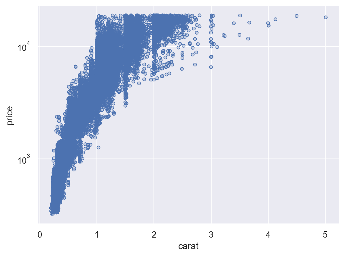
"log"or"symlog"will set the scale’s transform:p1 = so.Plot(diamonds, x="carat", y="price") p1.add(so.Dots()).scale(y="log")
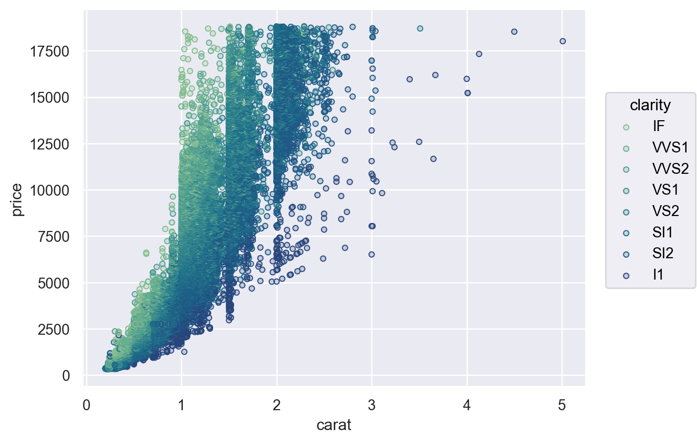
String arguments can also specify the the name of a palette that defines the output values (or “range”) of the scale:
p1.add(so.Dots(), color="clarity").scale(color="crest")
The scale’s range can alternatively be specified as a tuple of min/max values:
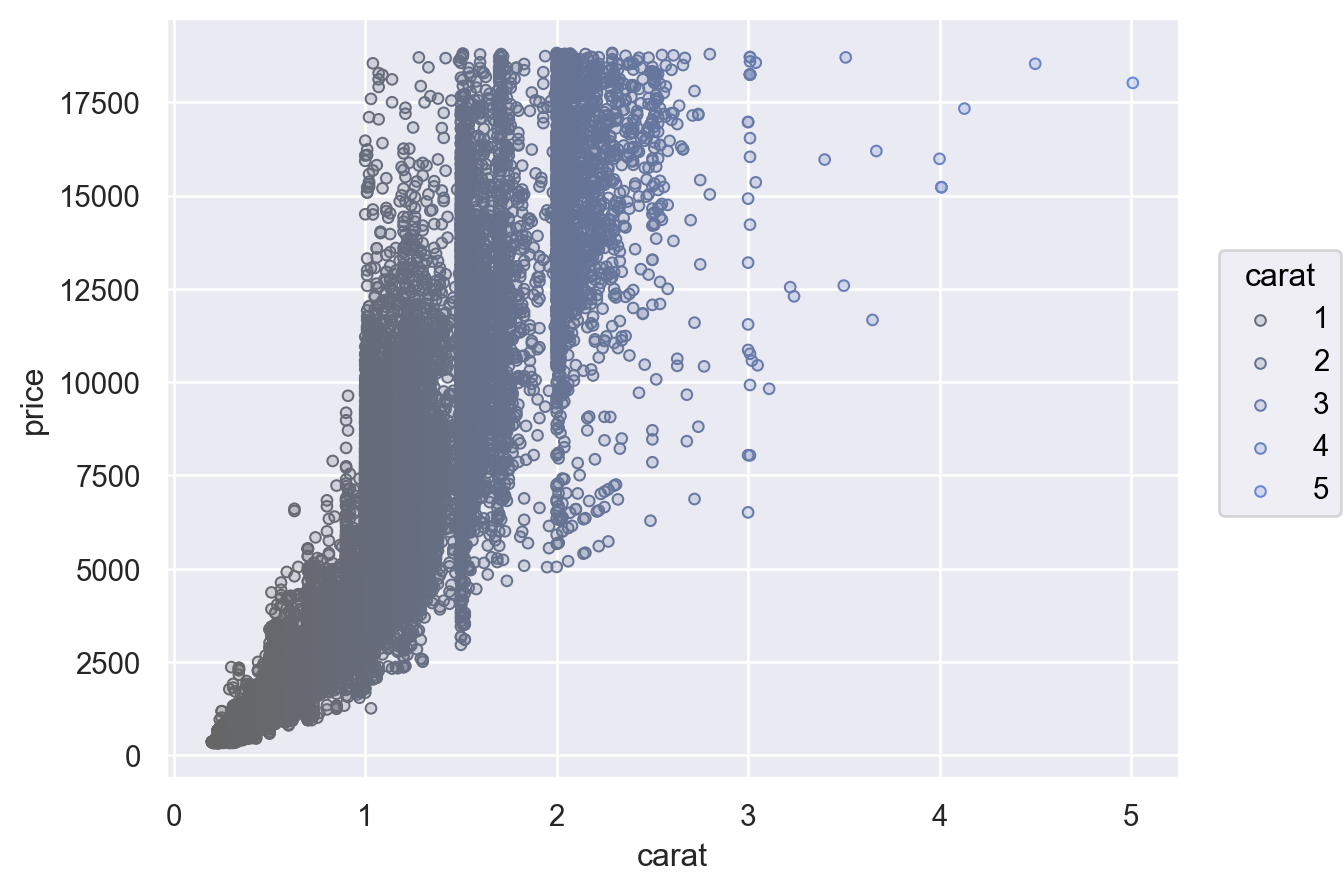
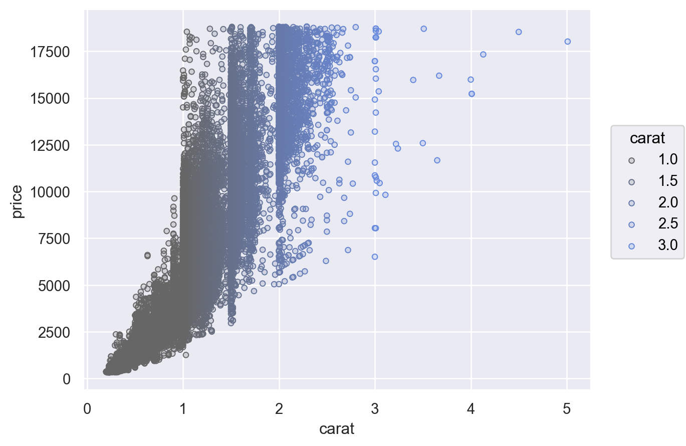
p1.add(so.Dots(), pointsize="carat").scale(pointsize=(2, 10))

The tuple format can also be used for a color scale:
p1.add(so.Dots(), color="carat").scale(color=(".4", "#68d"))
For more control pass a scale object, such as
Continuous, which allows you to specify the input domain (norm), output range (values), and nonlinear transform (trans):( p1.add(so.Dots(), color="carat") .scale(color=so.Continuous((".4", "#68d"), norm=(1, 3), trans="sqrt")) )
The scale objects also offer an interface for configuring the location of the scale ticks (including in the legend) and the formatting of the tick labels:
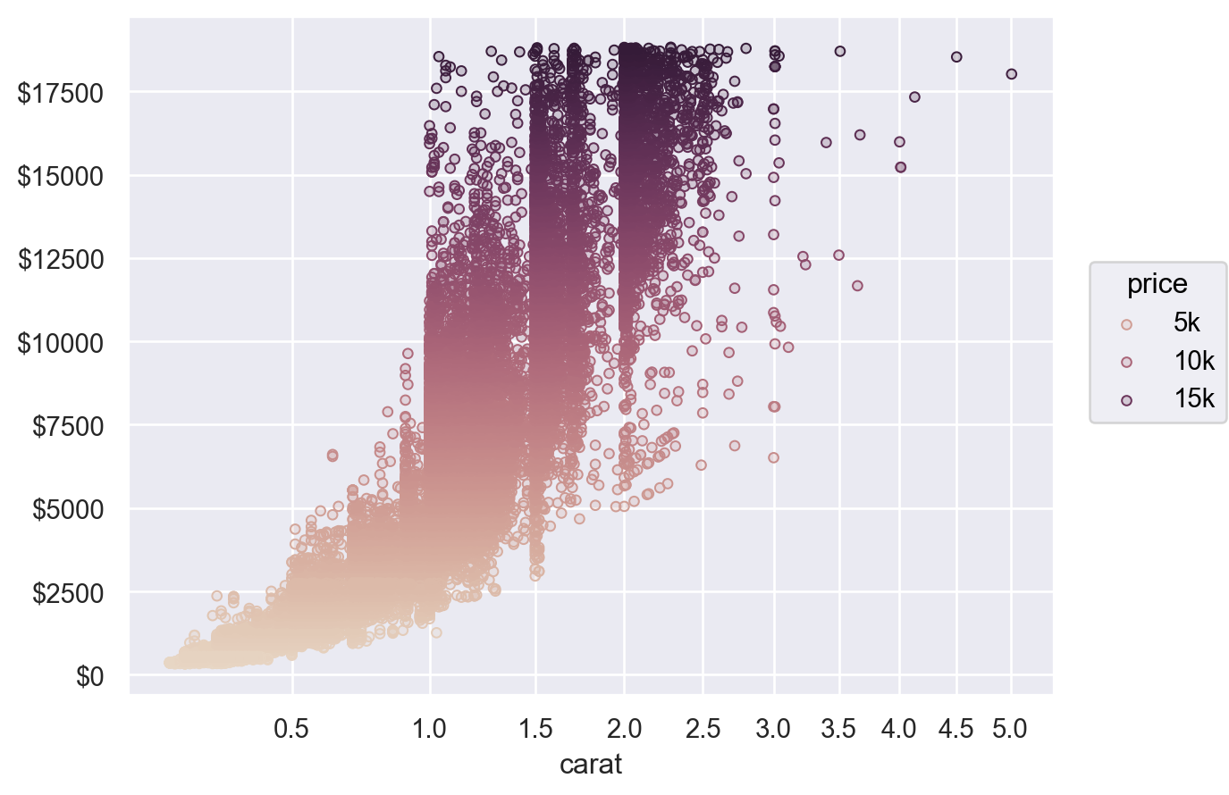
(
    p1.add(so.Dots(), color="price")
    .scale(
        x=so.Continuous(trans="sqrt").tick(every=.5),
        y=so.Continuous().label(like="${x:g}"),
        color=so.Continuous("ch:.2").tick(upto=4).label(unit=""),
    )
    .label(y="")
)
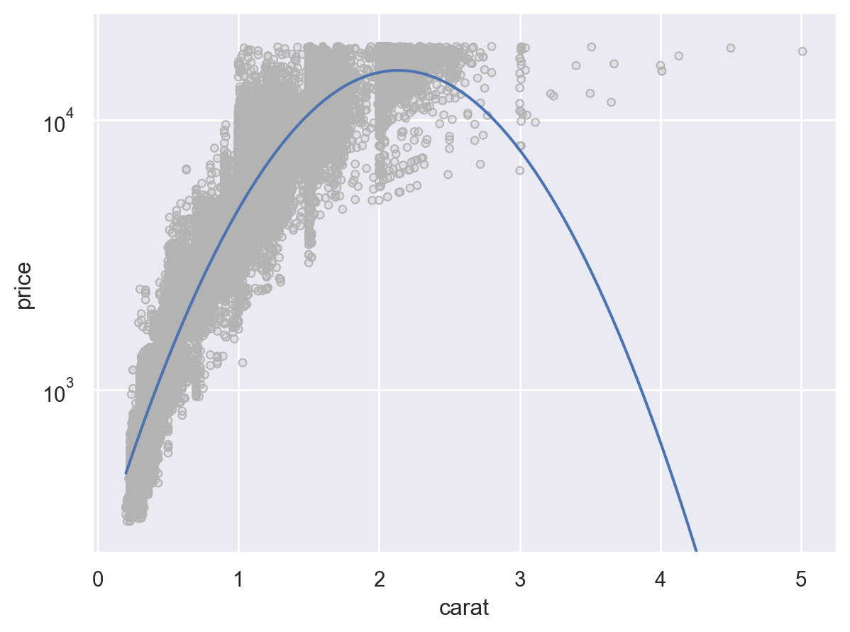
If the scale includes a nonlinear transform, it will be applied before any statistical transforms:
(
    p1.add(so.Dots(color=".7"))
    .add(so.Line(), so.PolyFit(order=2))
    .scale(y="log")
    .limit(y=(250, 25000))
)
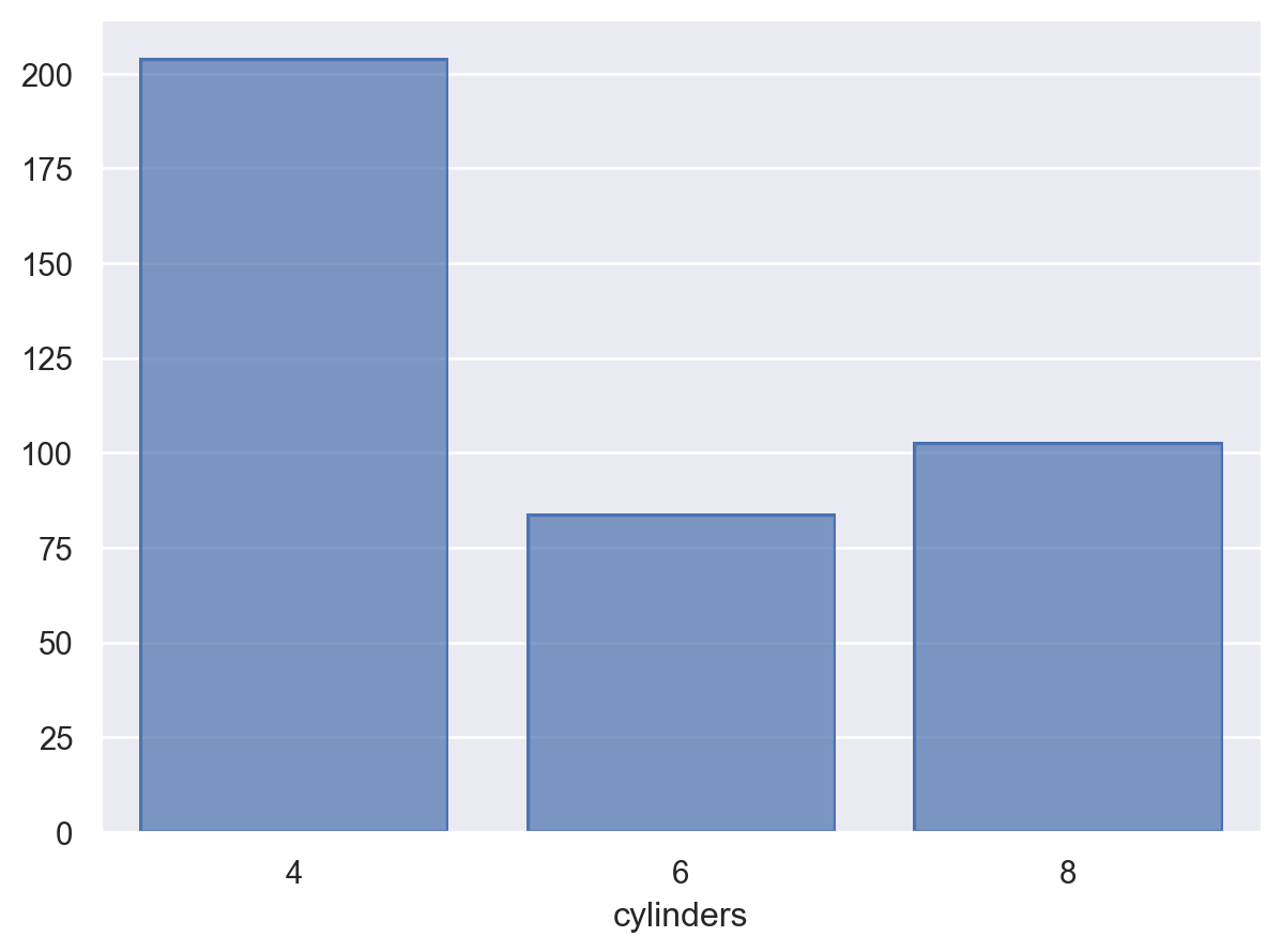
The scale is also relevant for when numerical data should be treated as categories. Consider the following histogram:
p2 = so.Plot(mpg, "cylinders").add(so.Bar(), so.Hist())
p2
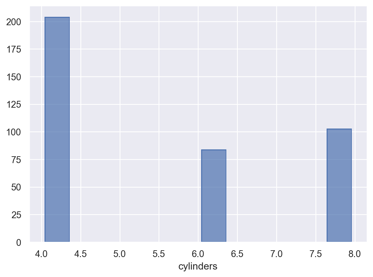
By default, the plot gives
cylindersa continuous scale, since it is a vector of floats. But assigning aNominalscale causes the histogram to bin observations properly:p2.scale(x=so.Nominal())
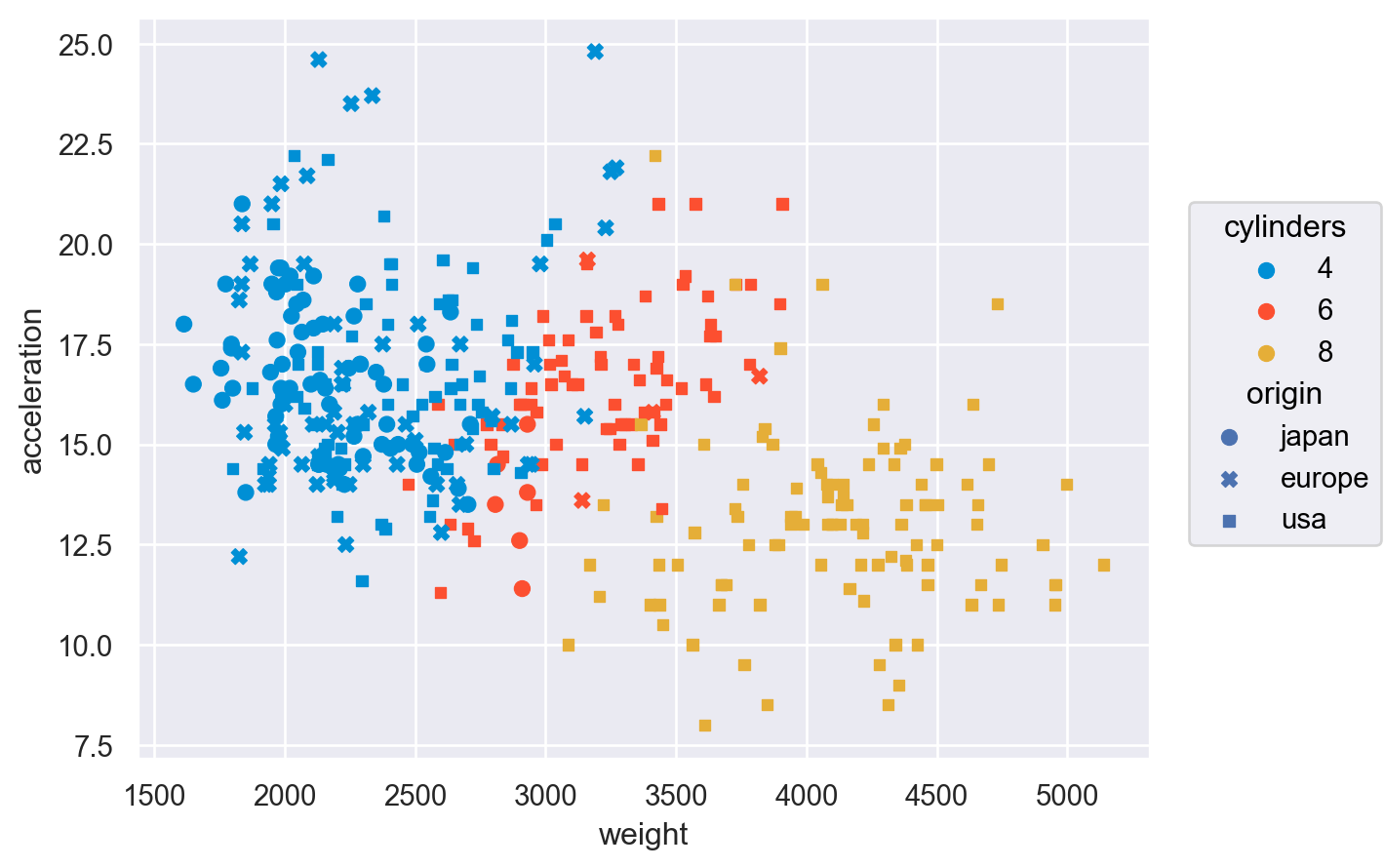
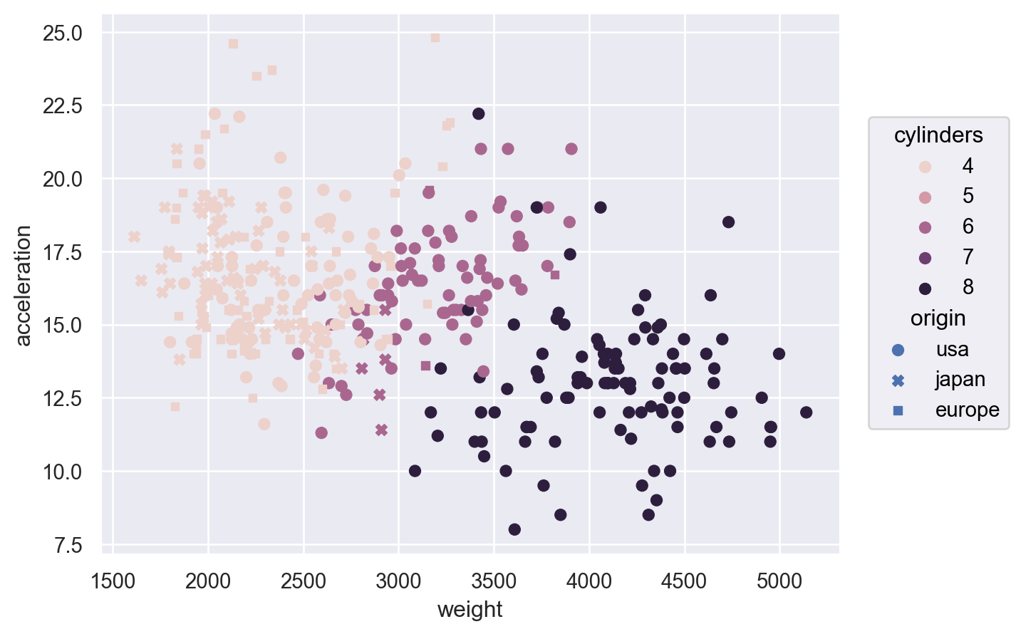
The default behavior for semantic mappings also depends on input data types and can be modified by the scale. Consider the sequential mapping applied to the colors in this plot:
p3 = (
    so.Plot(mpg, "weight", "acceleration", color="cylinders")
    .add(so.Dot(), marker="origin")
)
p3
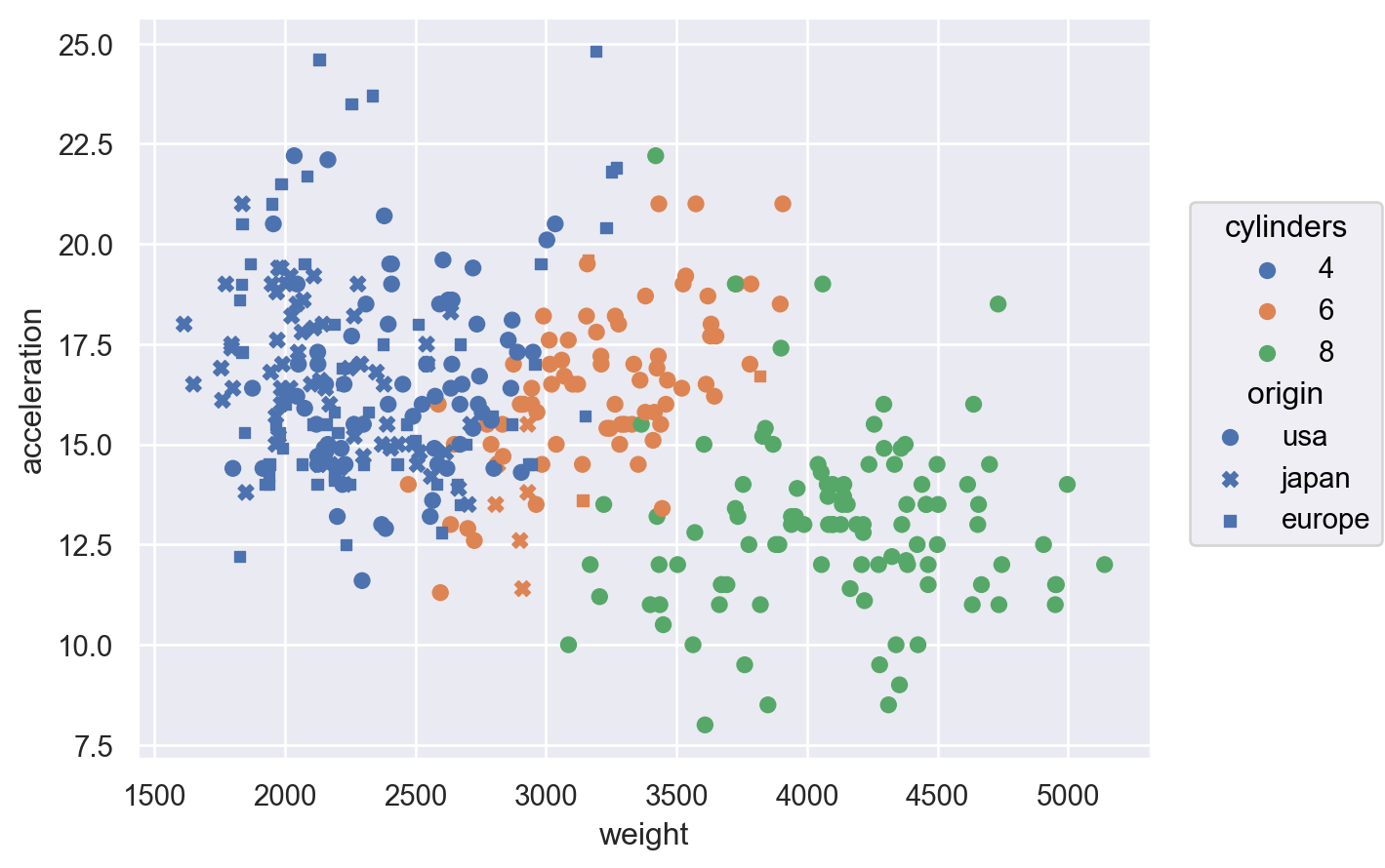
Passing the name of a qualitative palette will select a
Nominalscale:p3.scale(color="deep")
A
Nominalscale is also implied when the output values are given as a list or dictionary:p3.scale( color=["#49b", "#a6a", "#5b8"], marker={"japan": ".", "europe": "+", "usa": "*"}, )

Pass a
Nominalobject directly to control the order of the category mappings:p3.scale( color=so.Nominal(["#008fd5", "#fc4f30", "#e5ae38"]), marker=so.Nominal(order=["japan", "europe", "usa"]) )