seaborn.objects.KDE

class seaborn.objects.KDE(bw_adjust=1, bw_method='scott', common_norm=True, common_grid=True, gridsize=200, cut=3, cumulative=False)

Compute a univariate kernel density estimate.

Parameters:

bw_adjustfloat

Factor that multiplicatively scales the value chosen using bw_method. Increasing will make the curve smoother. See Notes.

bw_methodstring, scalar, or callable

Method for determining the smoothing bandwidth to use. Passed directly to scipy.stats.gaussian_kde; see there for options.

common_normbool or list of variables

If True, normalize so that the areas of all curves sums to 1. If False, normalize each curve independently. If a list, defines variable(s) to group by and normalize within.

common_gridbool or list of variables

If True, all curves will share the same evaluation grid. If False, each evaluation grid is independent. If a list, defines variable(s) to group by and share a grid within.

gridsizeint or None

Number of points in the evaluation grid. If None, the density is evaluated at the original datapoints.

cutfloat

Factor, multiplied by the kernel bandwidth, that determines how far the evaluation grid extends past the extreme datapoints. When set to 0, the curve is truncated at the data limits.

cumulativebool

If True, estimate a cumulative distribution function. Requires scipy.

Notes

The bandwidth, or standard deviation of the smoothing kernel, is an important parameter. Much like histogram bin width, using the wrong bandwidth can produce a distorted representation. Over-smoothing can erase true features, while under-smoothing can create false ones. The default uses a rule-of-thumb that works best for distributions that are roughly bell-shaped. It is a good idea to check the default by varying bw_adjust.

Because the smoothing is performed with a Gaussian kernel, the estimated density curve can extend to values that may not make sense. For example, the curve may be drawn over negative values when data that are naturally positive. The cut parameter can be used to control the evaluation range, but datasets that have many observations close to a natural boundary may be better served by a different method.

Similar distortions may arise when a dataset is naturally discrete or “spiky” (containing many repeated observations of the same value). KDEs will always produce a smooth curve, which could be misleading.

The units on the density axis are a common source of confusion. While kernel density estimation produces a probability distribution, the height of the curve at each point gives a density, not a probability. A probability can be obtained only by integrating the density across a range. The curve is normalized so that the integral over all possible values is 1, meaning that the scale of the density axis depends on the data values.

If scipy is installed, its cython-accelerated implementation will be used.

Examples

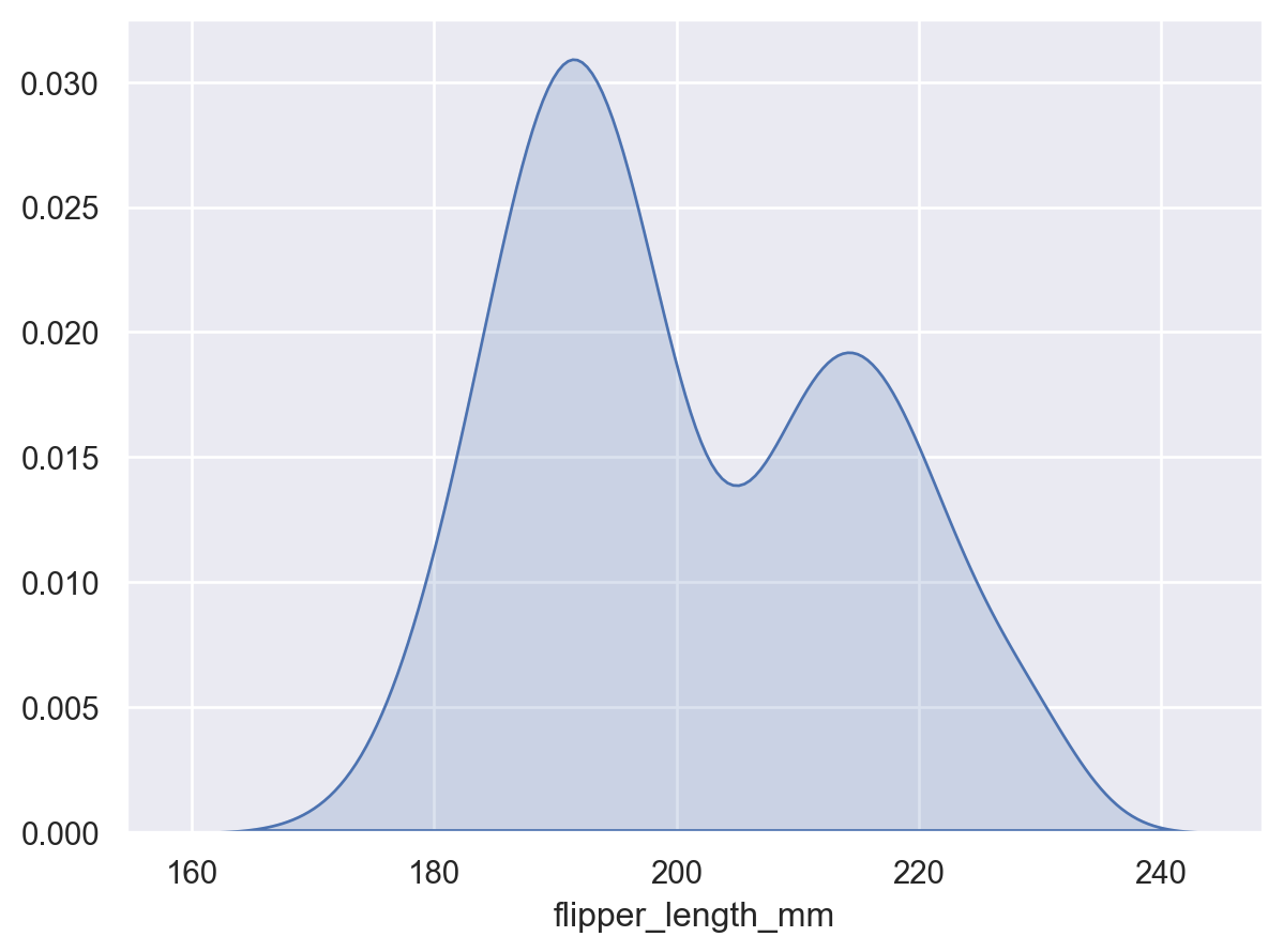
This stat estimates transforms observations into a smooth function representing the estimated density:

p = so.Plot(penguins, x="flipper_length_mm")
p.add(so.Area(), so.KDE())

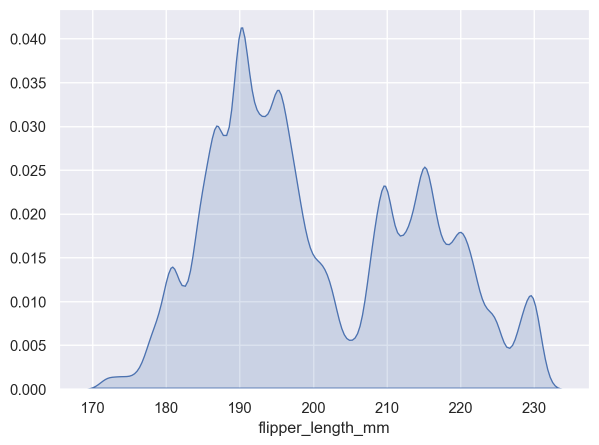
Adjust the smoothing bandwidth to see more or fewer details:

p.add(so.Area(), so.KDE(bw_adjust=0.25))

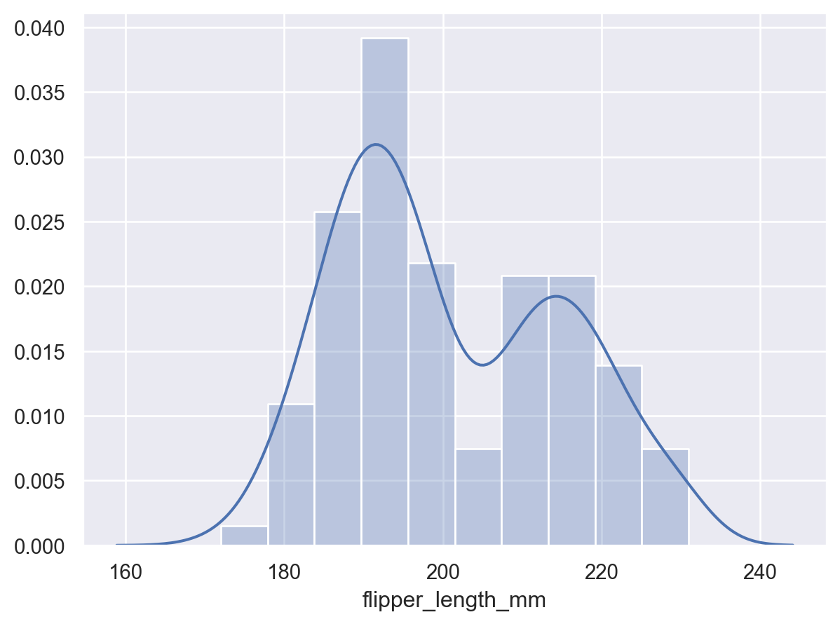
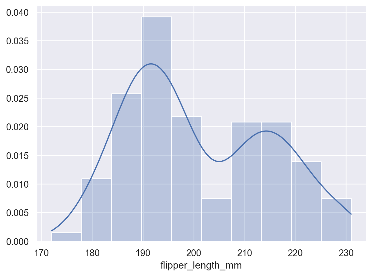
The curve will extend beyond observed values in the dataset:

p2 = p.add(so.Bars(alpha=.3), so.Hist("density"))
p2.add(so.Line(), so.KDE())

Control the range of the density curve relative to the observations using cut:

p2.add(so.Line(), so.KDE(cut=0))

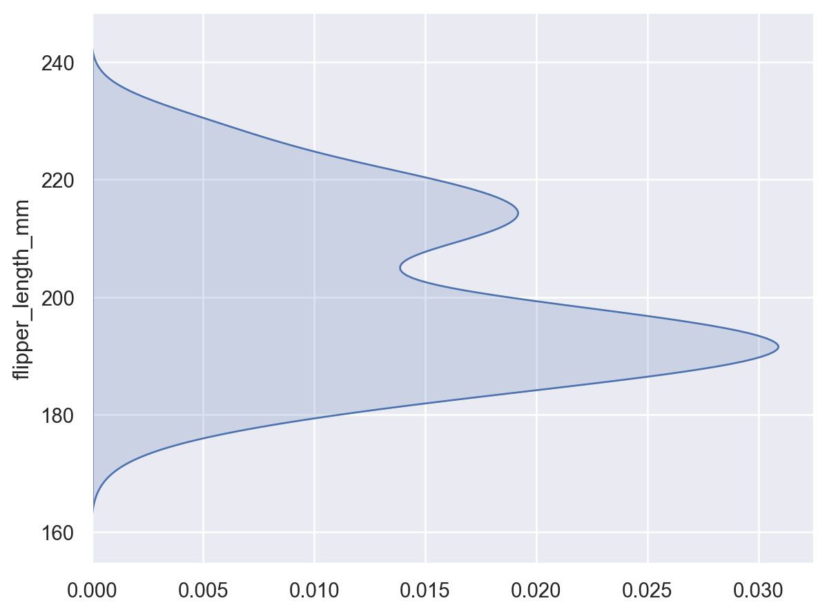
When observations are assigned to the y variable, the density will be shown for x:

so.Plot(penguins, y="flipper_length_mm").add(so.Area(), so.KDE())

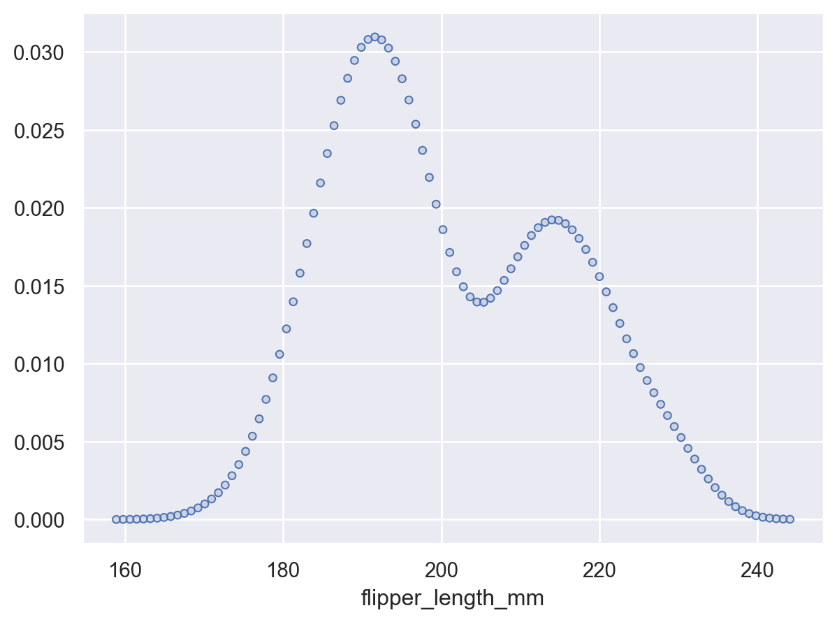
Use gridsize to increase or decrease the resolution of the grid where the density is evaluated:

p.add(so.Dots(), so.KDE(gridsize=100))

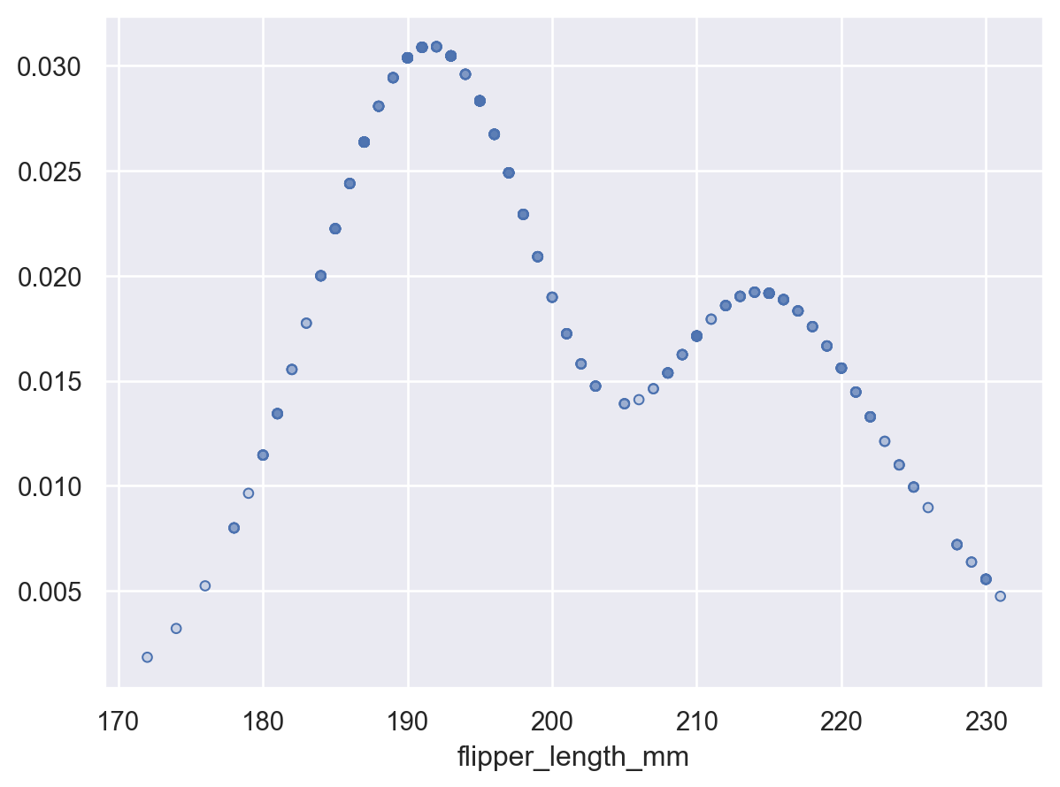
Or pass None to evaluate the density at the original datapoints:

p.add(so.Dots(), so.KDE(gridsize=None))

Other variables will define groups for the estimation:

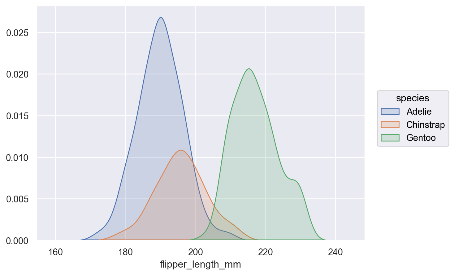
p.add(so.Area(), so.KDE(), color="species")

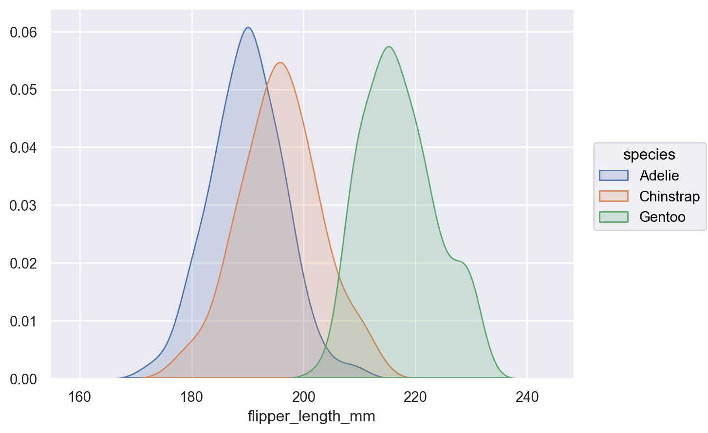
By default, the density is normalized across all groups (i.e., the joint density is shown); pass common_norm=False to show conditional densities:

p.add(so.Area(), so.KDE(common_norm=False), color="species")

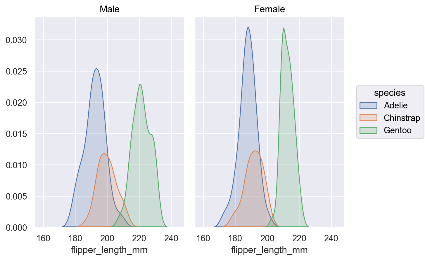
Or pass a list of variables to condition on:

(
    p.facet("sex")
    .add(so.Area(), so.KDE(common_norm=["col"]), color="species")
)

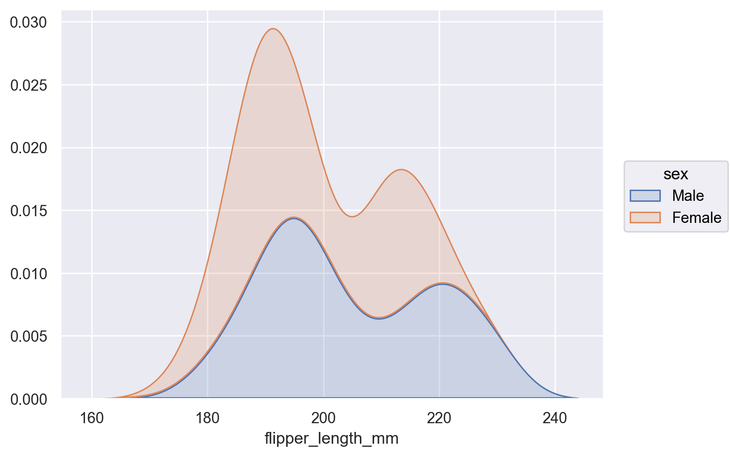
This stat can be combined with other transforms, such as Stack (when common_grid=True):

p.add(so.Area(), so.KDE(), so.Stack(), color="sex")

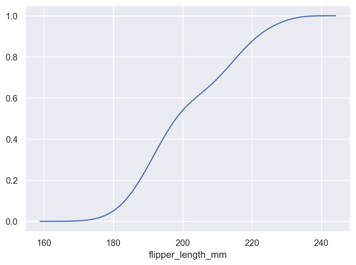
Set cumulative=True to integrate the density:

p.add(so.Line(), so.KDE(cumulative=True))