seaborn.objects.Plot.add#
- Plot.add(mark, *transforms, orient=None, legend=True, label=None, data=None, **variables)#
Specify a layer of the visualization in terms of mark and data transform(s).
This is the main method for specifying how the data should be visualized. It can be called multiple times with different arguments to define a plot with multiple layers.
- Parameters:
- mark
Mark The visual representation of the data to use in this layer.
- transforms
StatorMove Objects representing transforms to be applied before plotting the data. Currently, at most one
Statcan be used, and it must be passed first. This constraint will be relaxed in the future.- orient“x”, “y”, “v”, or “h”
The orientation of the mark, which also affects how transforms are computed. Typically corresponds to the axis that defines groups for aggregation. The “v” (vertical) and “h” (horizontal) options are synonyms for “x” / “y”, but may be more intuitive with some marks. When not provided, an orientation will be inferred from characteristics of the data and scales.
- legendbool
Option to suppress the mark/mappings for this layer from the legend.
- labelstr
A label to use for the layer in the legend, independent of any mappings.
- dataDataFrame or dict
Data source to override the global source provided in the constructor.
- variablesdata vectors or identifiers
Additional layer-specific variables, including variables that will be passed directly to the transforms without scaling.
- mark
Examples
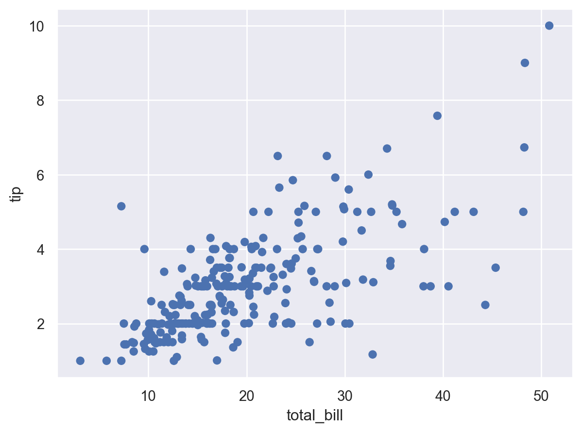
Every layer must be defined with a
Mark:p = so.Plot(tips, "total_bill", "tip").add(so.Dot()) p
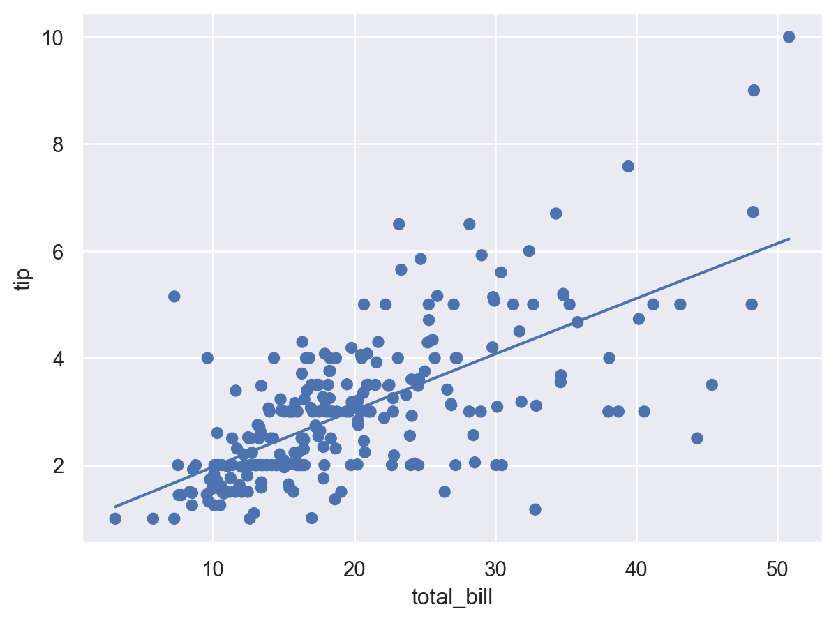
Call
Plot.addmultiple times to add multiple layers. In addition to theMark, layers can also be defined withStatorMovetransforms:p.add(so.Line(), so.PolyFit())
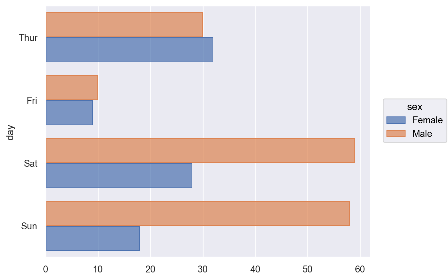
Multiple transforms can be stacked into a pipeline.
(
    so.Plot(tips, y="day", color="sex")
    .add(so.Bar(), so.Hist(), so.Dodge())
)
Layers have an “orientation”, which affects the transforms and some marks. The orientation is typically inferred from the variable types assigned to
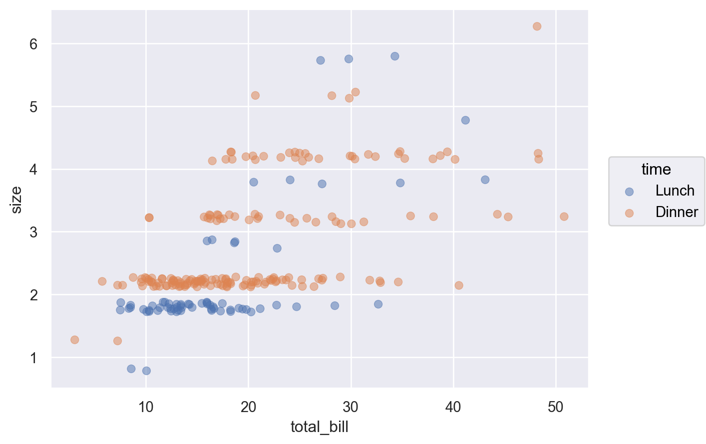
xandy, but it can be specified when it would otherwise be ambiguous:( so.Plot(tips, x="total_bill", y="size", color="time") .add(so.Dot(alpha=.5), so.Dodge(), so.Jitter(.4), orient="y") )
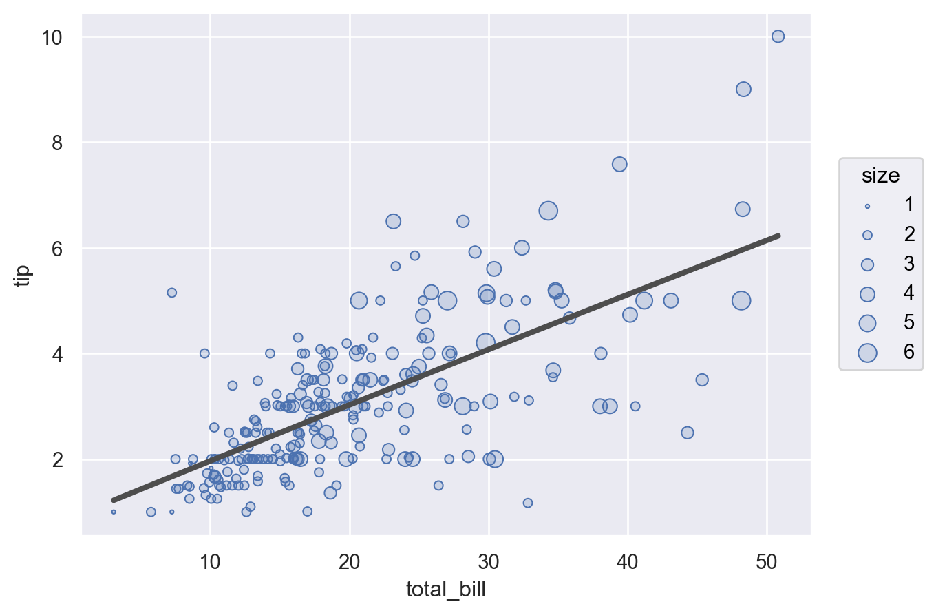
Variables can be assigned to a specific layer. Note the distinction between how
pointsizeis passed toPlot.add— so it is mapped by a scale — whilecolorandlinewidthare passed directly toLine, so they directly set the line’s color and width:( so.Plot(tips, "total_bill", "tip") .add(so.Dots(), pointsize="size") .add(so.Line(color=".3", linewidth=3), so.PolyFit()) .scale(pointsize=(2, 10)) )
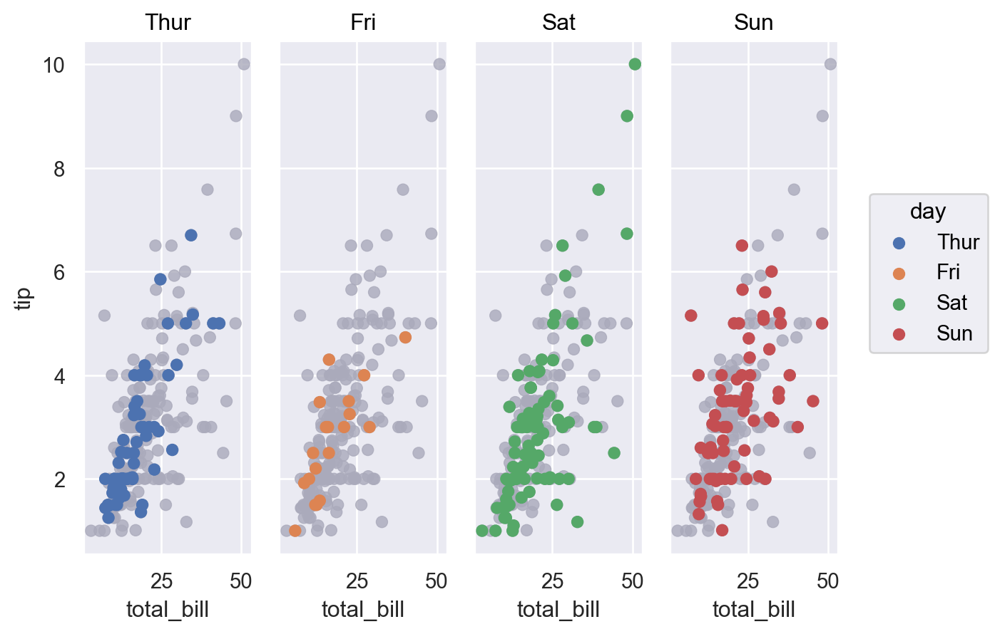
Variables that would otherwise apply to the entire plot can also be excluded from a specific layer by setting their value to
None:( so.Plot(tips, "total_bill", "tip", color="day") .facet(col="day") .add(so.Dot(color="#aabc"), col=None, color=None) .add(so.Dot()) )
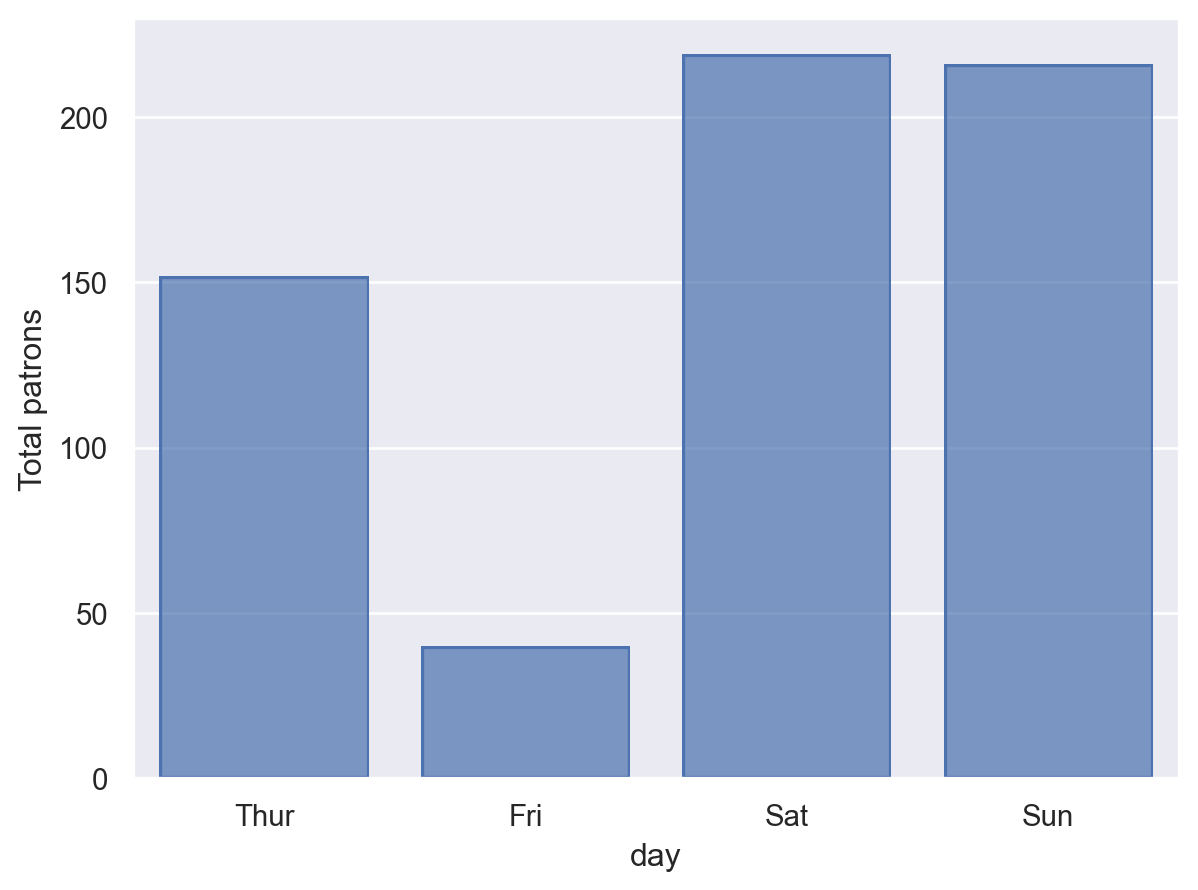
Variables used only by the transforms must be passed at the layer level:
(
    so.Plot(tips, "day")
    .add(so.Bar(), so.Hist(), weight="size")
    .label(y="Total patrons")
)
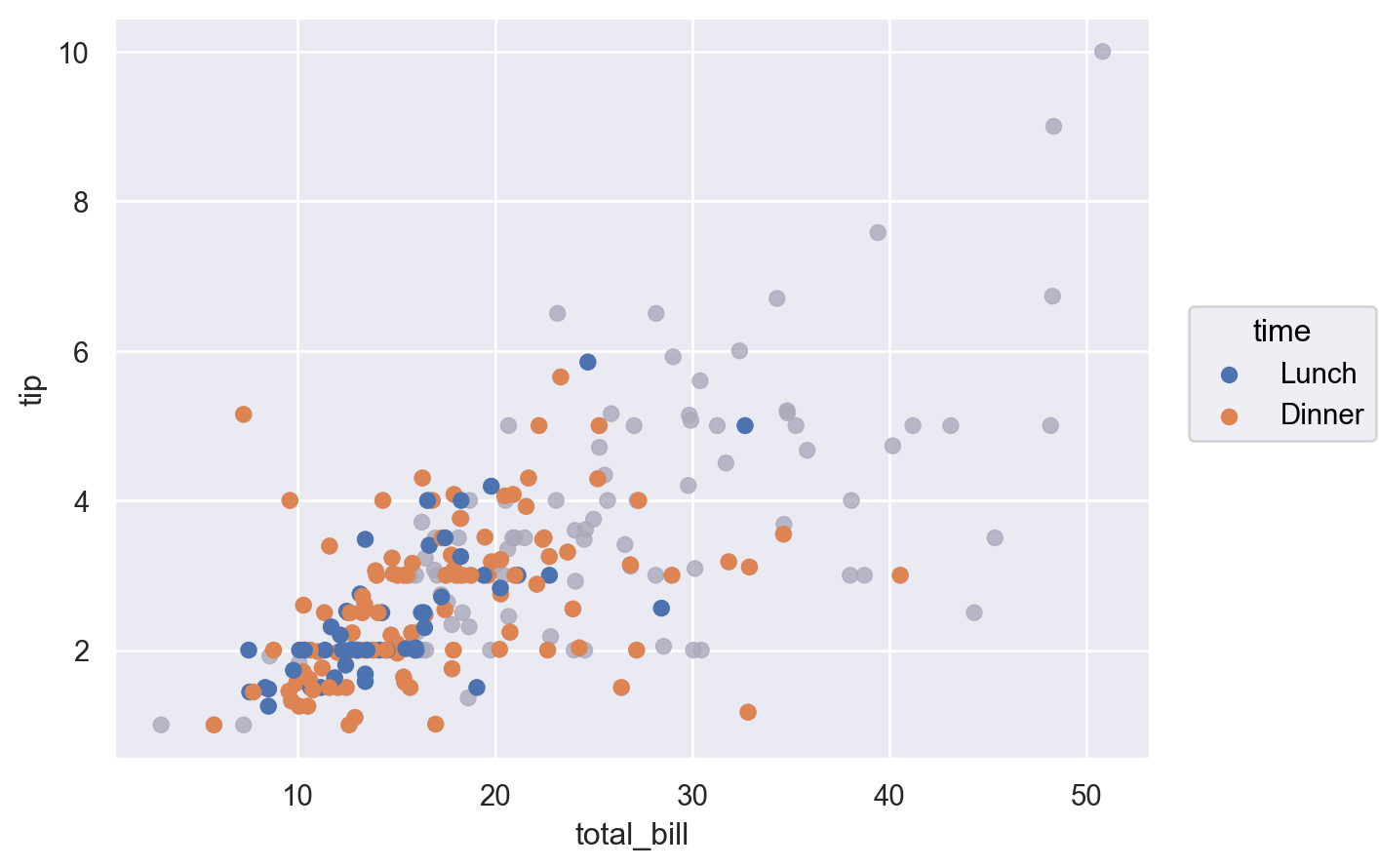
Each layer can be provided with its own data source. If a data source was provided in the constructor, the layer data will be joined using its index:
(
    so.Plot(tips, "total_bill", "tip")
    .add(so.Dot(color="#aabc"))
    .add(so.Dot(), data=tips.query("size == 2"), color="time")
)
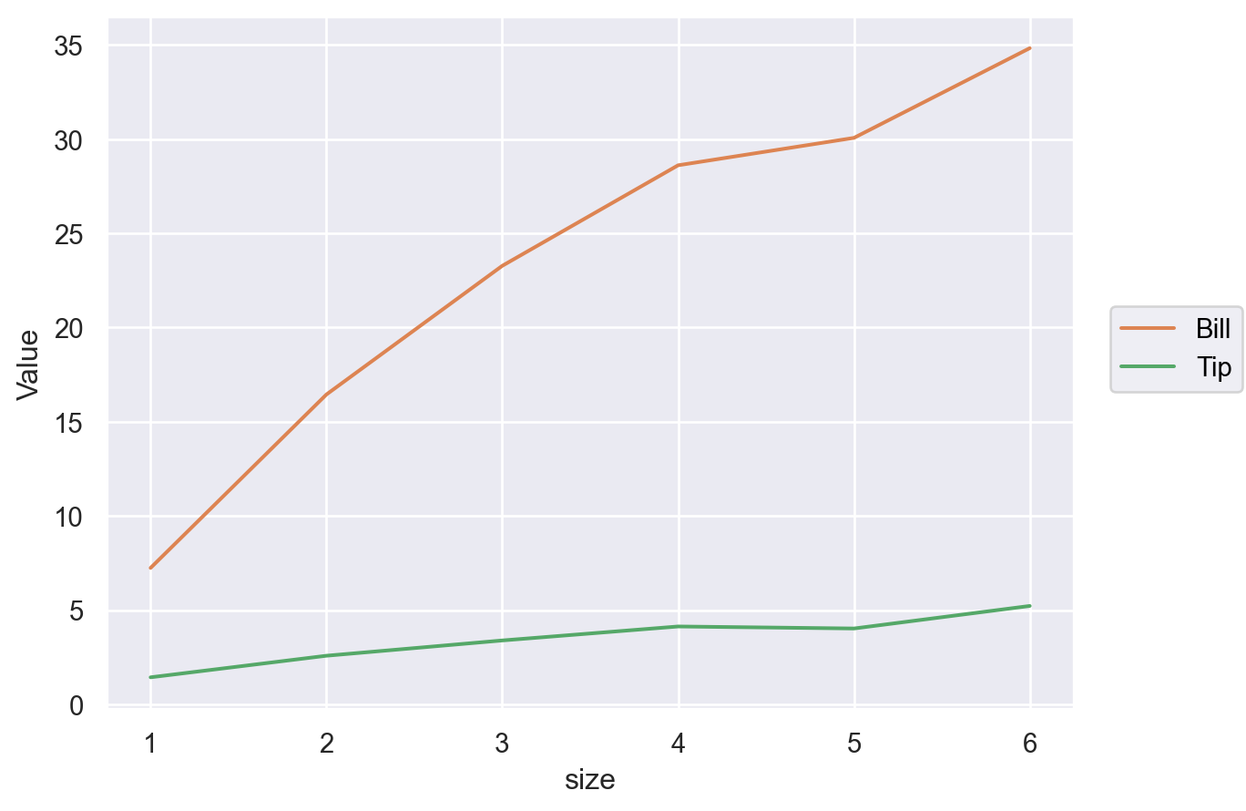
Providing a
labelwill annotate the layer in the plot’s legend:( so.Plot(tips, x="size") .add(so.Line(color="C1"), so.Agg(), y="total_bill", label="Bill") .add(so.Line(color="C2"), so.Agg(), y="tip", label="Tip") .label(y="Value") )