seaborn.objects.Hist

class seaborn.objects.Hist(stat='count', bins='auto', binwidth=None, binrange=None, common_norm=True, common_bins=True, cumulative=False, discrete=False)

Bin observations, count them, and optionally normalize or cumulate.

Parameters:

statstr

Aggregate statistic to compute in each bin:

• count: the number of observations

• density: normalize so that the total area of the histogram equals 1

• percent: normalize so that bar heights sum to 100

• probability or proportion: normalize so that bar heights sum to 1

• frequency: divide the number of observations by the bin width

binsstr, int, or ArrayLike

Generic parameter that can be the name of a reference rule, the number of bins, or the bin breaks. Passed to numpy.histogram_bin_edges().

binwidthfloat

Width of each bin; overrides bins but can be used with binrange. Note that if binwidth does not evenly divide the bin range, the actual bin width used will be only approximately equal to the parameter value.

binrange(min, max)

Lowest and highest value for bin edges; can be used with either bins (when a number) or binwidth. Defaults to data extremes.

common_normbool or list of variables

When not False, the normalization is applied across groups. Use True to normalize across all groups, or pass variable name(s) that define normalization groups.

common_binsbool or list of variables

When not False, the same bins are used for all groups. Use True to share bins across all groups, or pass variable name(s) to share within.

cumulativebool

If True, cumulate the bin values.

discretebool

If True, set binwidth and binrange so that bins have unit width and are centered on integer values

Notes

The choice of bins for computing and plotting a histogram can exert substantial influence on the insights that one is able to draw from the visualization. If the bins are too large, they may erase important features. On the other hand, bins that are too small may be dominated by random variability, obscuring the shape of the true underlying distribution. The default bin size is determined using a reference rule that depends on the sample size and variance. This works well in many cases, (i.e., with “well-behaved” data) but it fails in others. It is always a good to try different bin sizes to be sure that you are not missing something important. This function allows you to specify bins in several different ways, such as by setting the total number of bins to use, the width of each bin, or the specific locations where the bins should break.

Examples

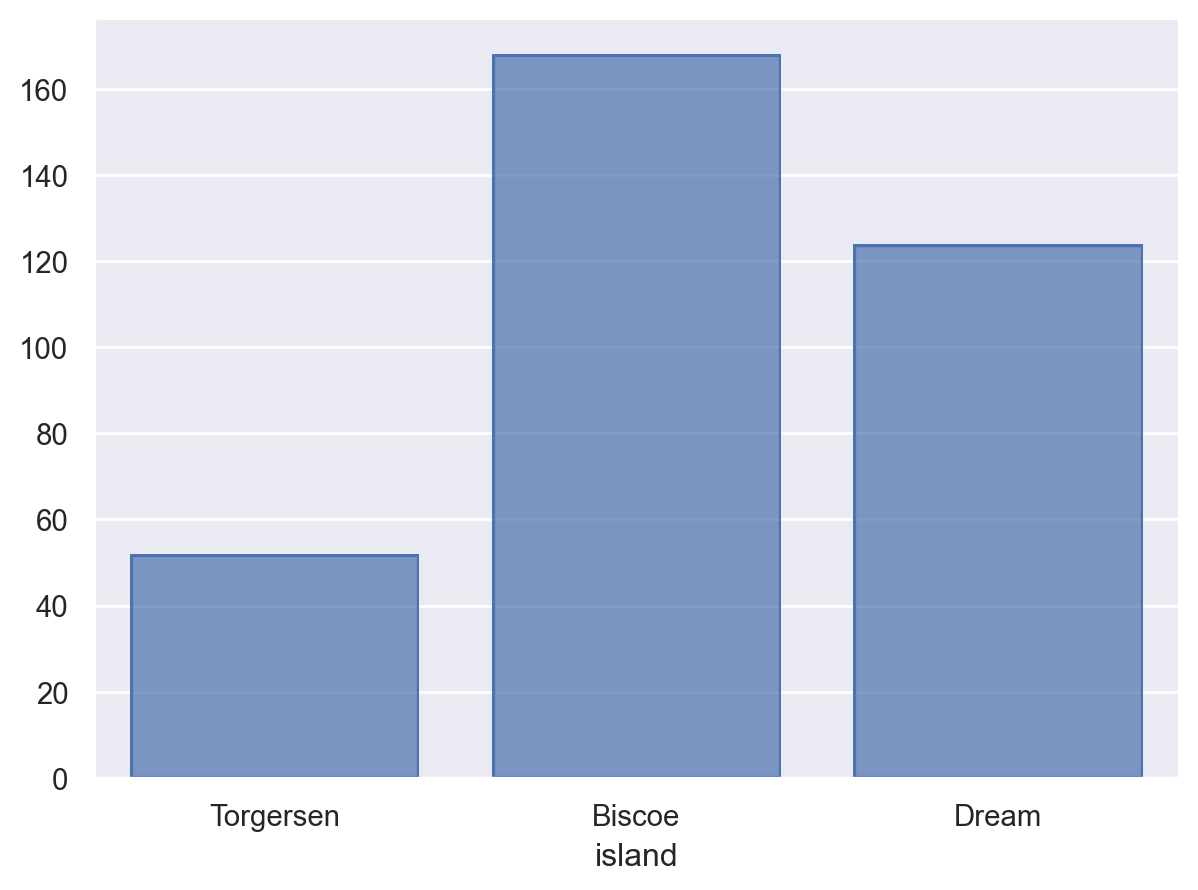
For discrete or categorical variables, this stat is commonly combined with a Bar mark:

so.Plot(penguins, "island").add(so.Bar(), so.Hist())

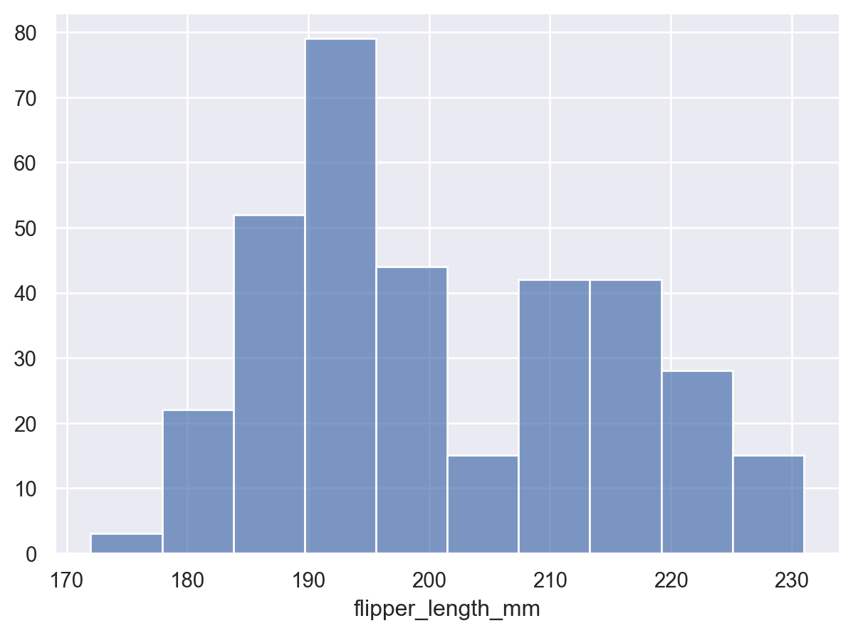
When used to estimate a univariate distribution, it is better to use the Bars mark:

p = so.Plot(penguins, "flipper_length_mm")
p.add(so.Bars(), so.Hist())

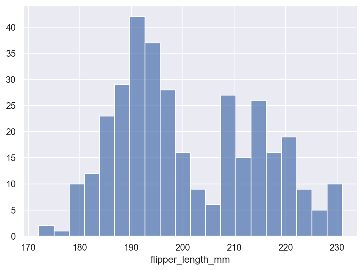
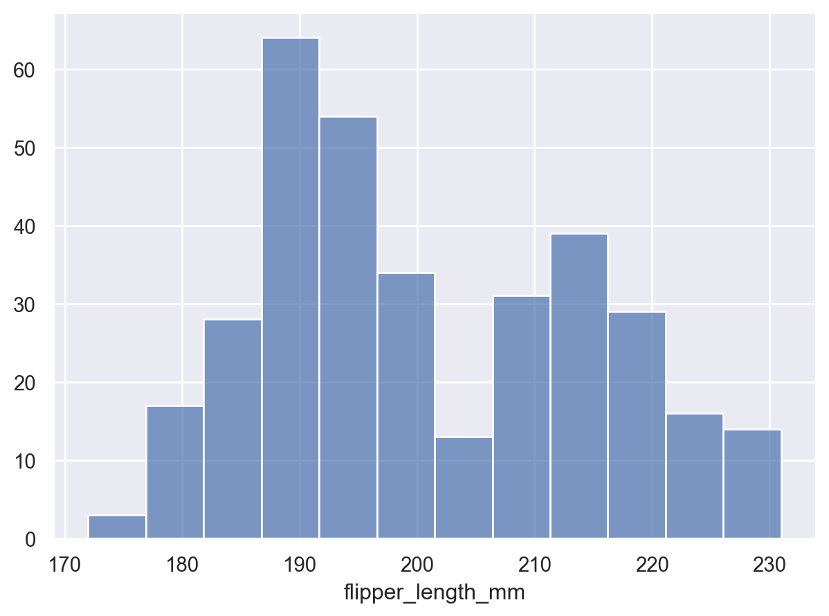
The granularity of the bins will influence whether the underlying distribution is accurately represented. Adjust it by setting the total number:

p.add(so.Bars(), so.Hist(bins=20))

Alternatively, specify the width of the bins:

p.add(so.Bars(), so.Hist(binwidth=5))

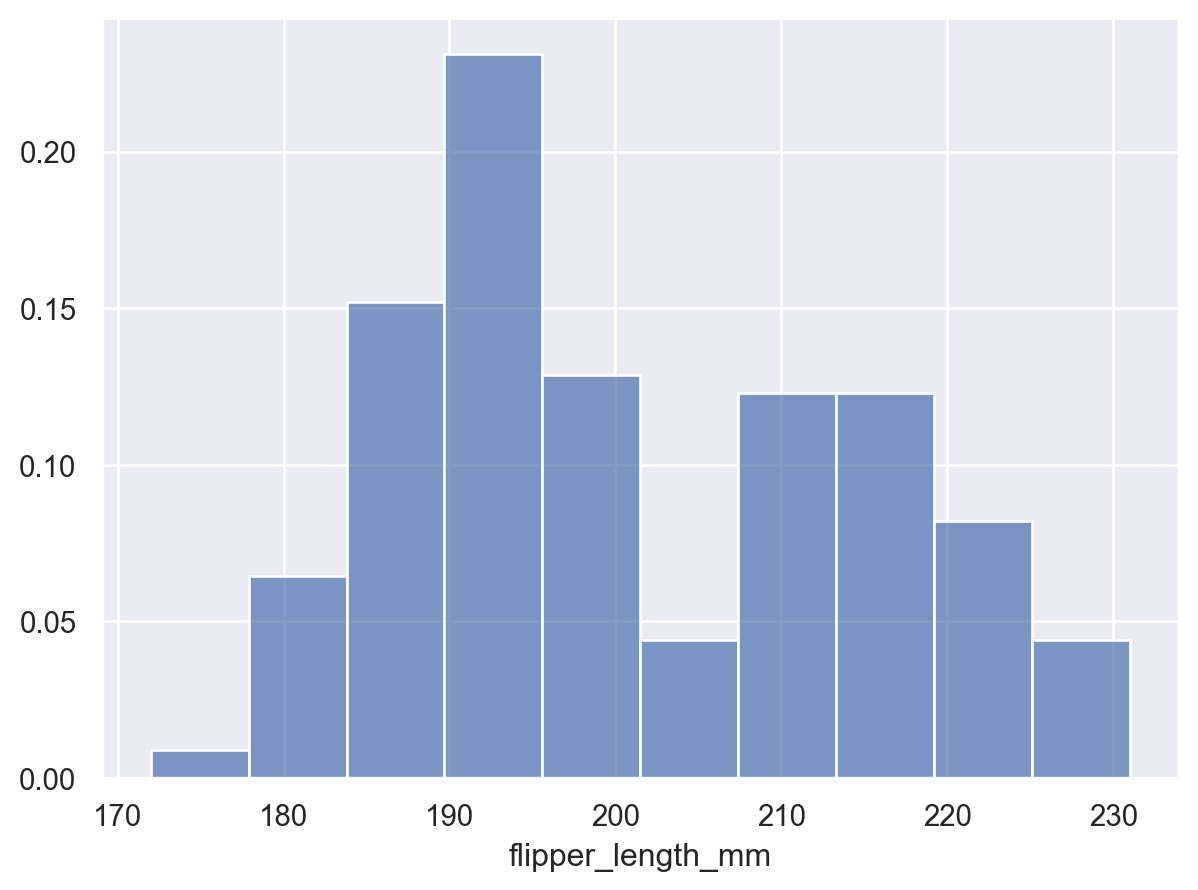
By default, the transform returns the count of observations in each bin. The counts can be normalized, e.g. to show a proportion:

p.add(so.Bars(), so.Hist(stat="proportion"))

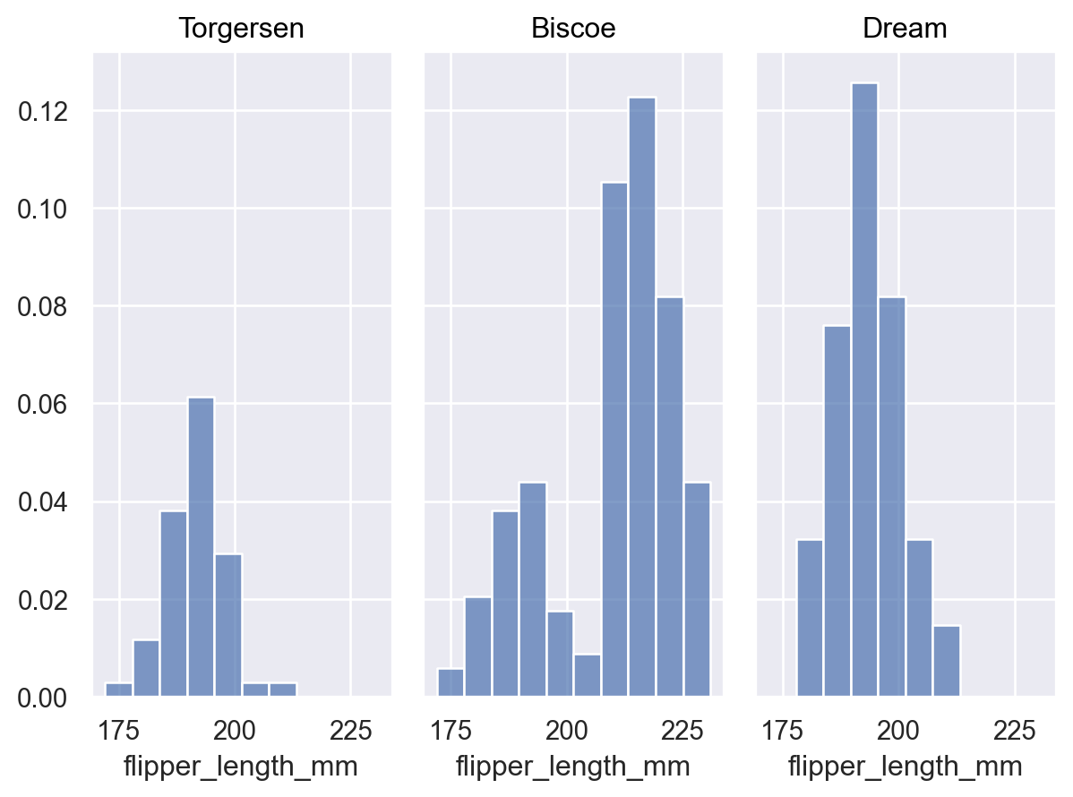
When additional variables define groups, the default behavior is to normalize across all groups:

p = p.facet("island")
p.add(so.Bars(), so.Hist(stat="proportion"))

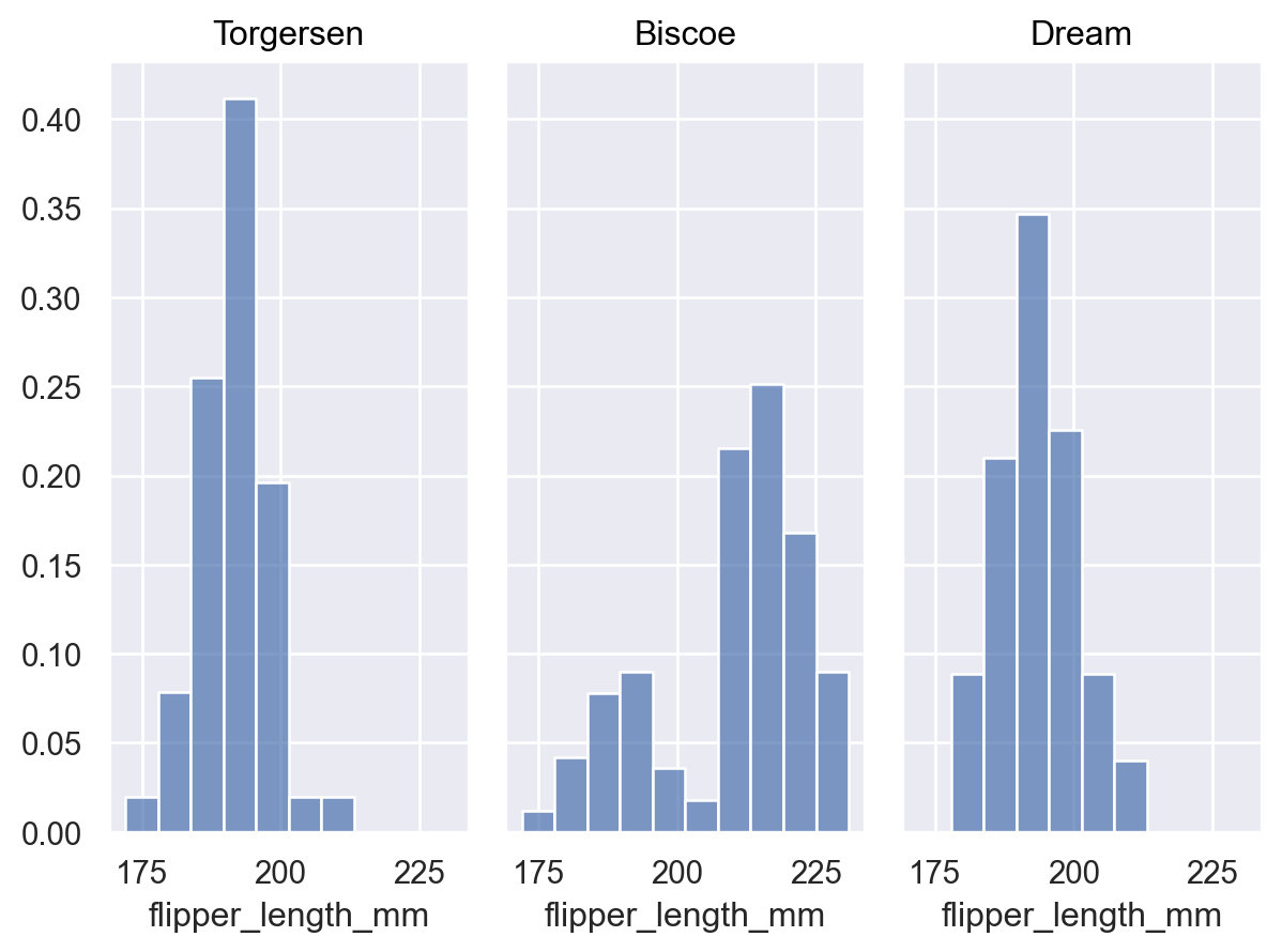
Pass common_norm=False to normalize each distribution independently:

p.add(so.Bars(), so.Hist(stat="proportion", common_norm=False))

Or, with more than one grouping varible, specify a subset to normalize within:

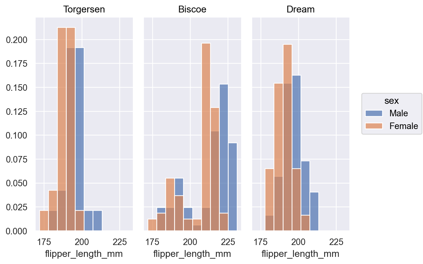
p.add(so.Bars(), so.Hist(stat="proportion", common_norm=["col"]), color="sex")

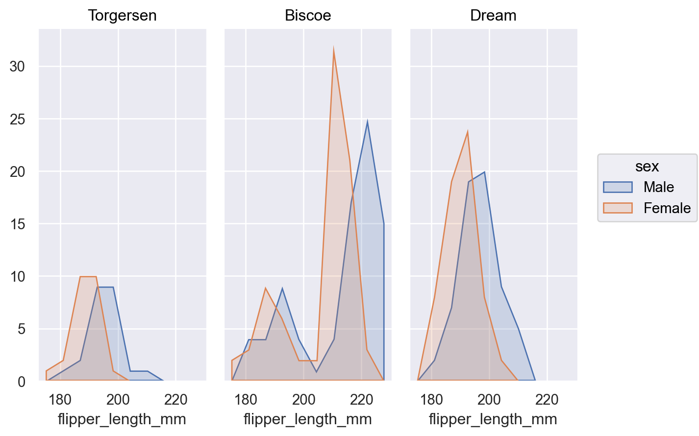
When distributions overlap it may be easier to discern their shapes with an Area mark:

p.add(so.Area(), so.Hist(), color="sex")

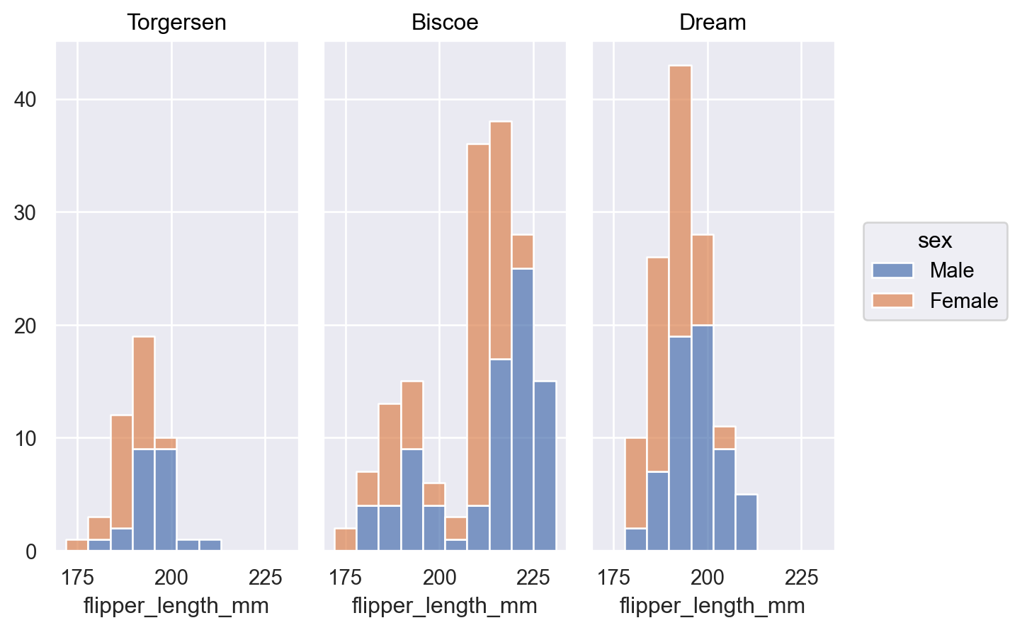
Or add Stack move to represent a part-whole relationship:

p.add(so.Bars(), so.Hist(), so.Stack(), color="sex")