seaborn.rugplot#
- seaborn.rugplot(data=None, *, x=None, y=None, hue=None, height=0.025, expand_margins=True, palette=None, hue_order=None, hue_norm=None, legend=True, ax=None, **kwargs)#
Plot marginal distributions by drawing ticks along the x and y axes.
This function is intended to complement other plots by showing the location of individual observations in an unobtrusive way.
- Parameters:
- data
pandas.DataFrame,numpy.ndarray, mapping, or sequence Input data structure. Either a long-form collection of vectors that can be assigned to named variables or a wide-form dataset that will be internally reshaped.
- x, yvectors or keys in
data Variables that specify positions on the x and y axes.
- huevector or key in
data Semantic variable that is mapped to determine the color of plot elements.
- heightfloat
Proportion of axes extent covered by each rug element. Can be negative.
- expand_marginsbool
If True, increase the axes margins by the height of the rug to avoid overlap with other elements.
- palettestring, list, dict, or
matplotlib.colors.Colormap Method for choosing the colors to use when mapping the
huesemantic. String values are passed tocolor_palette(). List or dict values imply categorical mapping, while a colormap object implies numeric mapping.- hue_ordervector of strings
Specify the order of processing and plotting for categorical levels of the
huesemantic.- hue_normtuple or
matplotlib.colors.Normalize Either a pair of values that set the normalization range in data units or an object that will map from data units into a [0, 1] interval. Usage implies numeric mapping.
- legendbool
If False, do not add a legend for semantic variables.
- ax
matplotlib.axes.Axes Pre-existing axes for the plot. Otherwise, call
matplotlib.pyplot.gca()internally.- kwargs
Other keyword arguments are passed to
matplotlib.collections.LineCollection()
- data
- Returns:
matplotlib.axes.AxesThe matplotlib axes containing the plot.
Examples
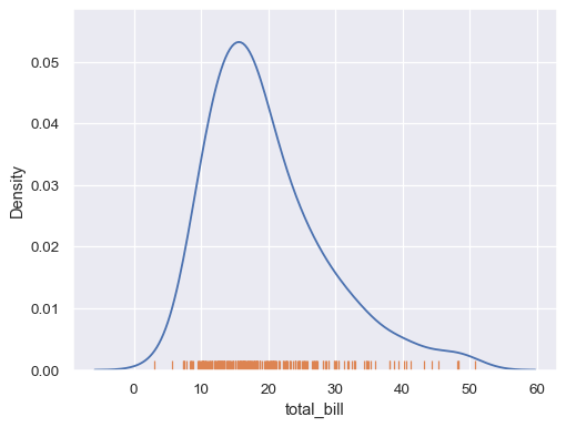
Add a rug along one of the axes:
import seaborn as sns; sns.set_theme()
tips = sns.load_dataset("tips")
sns.kdeplot(data=tips, x="total_bill")
sns.rugplot(data=tips, x="total_bill")
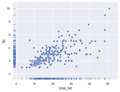
Add a rug along both axes:
sns.scatterplot(data=tips, x="total_bill", y="tip")
sns.rugplot(data=tips, x="total_bill", y="tip")
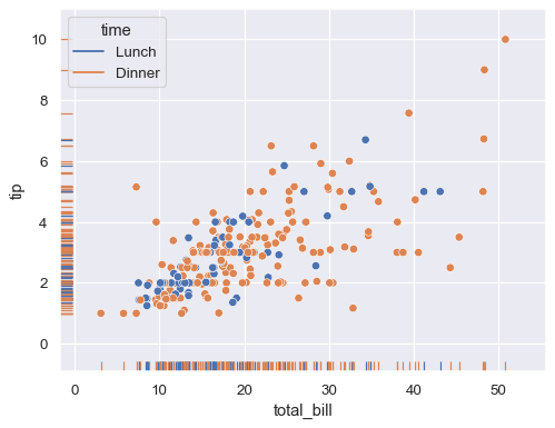
Represent a third variable with hue mapping:
sns.scatterplot(data=tips, x="total_bill", y="tip", hue="time")
sns.rugplot(data=tips, x="total_bill", y="tip", hue="time")
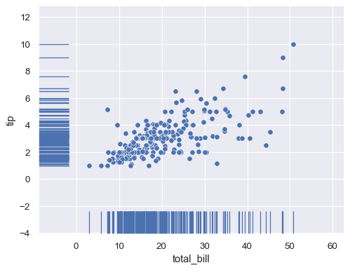
Draw a taller rug:
sns.scatterplot(data=tips, x="total_bill", y="tip")
sns.rugplot(data=tips, x="total_bill", y="tip", height=.1)
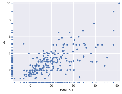
Put the rug outside the axes:
sns.scatterplot(data=tips, x="total_bill", y="tip")
sns.rugplot(data=tips, x="total_bill", y="tip", height=-.02, clip_on=False)
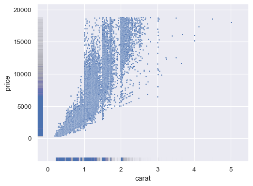
Show the density of a larger dataset using thinner lines and alpha blending:
diamonds = sns.load_dataset("diamonds")
sns.scatterplot(data=diamonds, x="carat", y="price", s=5)
sns.rugplot(data=diamonds, x="carat", y="price", lw=1, alpha=.005)
