seaborn.distplot
-
seaborn.distplot(a, bins=None, hist=True, kde=True, rug=False, fit=None, hist_kws=None, kde_kws=None, rug_kws=None, fit_kws=None, color=None, vertical=False, norm_hist=False, axlabel=None, label=None, ax=None)¶ Flexibly plot a univariate distribution of observations.
This function combines the matplotlib
histfunction (with automatic calculation of a good default bin size) with the seabornkdeplot()andrugplot()functions. It can also fitscipy.statsdistributions and plot the estimated PDF over the data.Parameters: a : Series, 1d-array, or list.
Observed data. If this is a Series object with a
nameattribute, the name will be used to label the data axis.bins : argument for matplotlib hist(), or None, optional
Specification of hist bins, or None to use Freedman-Diaconis rule.
hist : bool, optional
Whether to plot a (normed) histogram.
kde : bool, optional
Whether to plot a gaussian kernel density estimate.
rug : bool, optional
Whether to draw a rugplot on the support axis.
fit : random variable object, optional
An object with fit method, returning a tuple that can be passed to a pdf method a positional arguments following an grid of values to evaluate the pdf on.
{hist, kde, rug, fit}_kws : dictionaries, optional
Keyword arguments for underlying plotting functions.
color : matplotlib color, optional
Color to plot everything but the fitted curve in.
vertical : bool, optional
If True, observed values are on y-axis.
norm_hist : bool, optional
If True, the histogram height shows a density rather than a count. This is implied if a KDE or fitted density is plotted.
axlabel : string, False, or None, optional
Name for the support axis label. If None, will try to get it from a.namel if False, do not set a label.
label : string, optional
Legend label for the relevent component of the plot
ax : matplotlib axis, optional
if provided, plot on this axis
Returns: ax : matplotlib Axes
Returns the Axes object with the plot for further tweaking.
See also
Examples
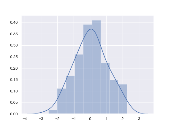
Show a default plot with a kernel density estimate and histogram with bin size determined automatically with a reference rule:
>>> import seaborn as sns, numpy as np
>>> sns.set(); np.random.seed(0)
>>> x = np.random.randn(100)
>>> ax = sns.distplot(x)
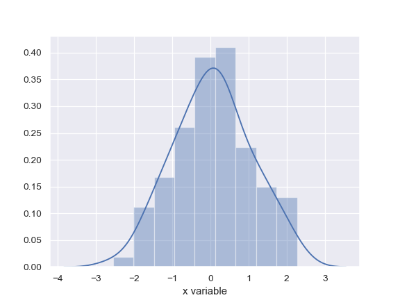
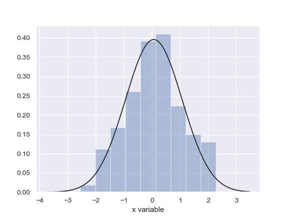
Use Pandas objects to get an informative axis label:
>>> import pandas as pd
>>> x = pd.Series(x, name="x variable")
>>> ax = sns.distplot(x)
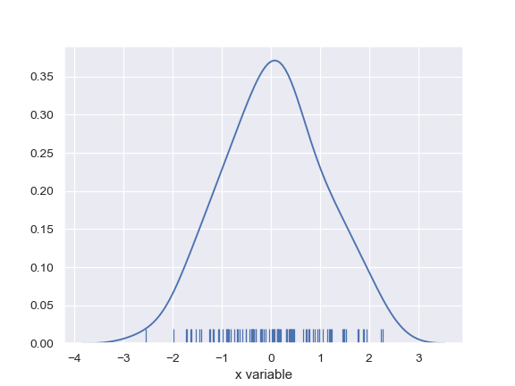
Plot the distribution with a kernel density estimate and rug plot:
>>> ax = sns.distplot(x, rug=True, hist=False)
Plot the distribution with a histogram and maximum likelihood gaussian distribution fit:
>>> from scipy.stats import norm
>>> ax = sns.distplot(x, fit=norm, kde=False)
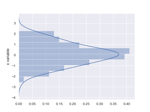
Plot the distribution on the vertical axis:
>>> ax = sns.distplot(x, vertical=True)
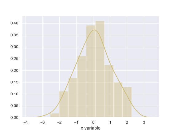
Change the color of all the plot elements:
>>> sns.set_color_codes()
>>> ax = sns.distplot(x, color="y")
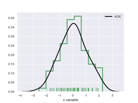
Pass specific parameters to the underlying plot functions:
>>> ax = sns.distplot(x, rug=True, rug_kws={"color": "g"},
...                   kde_kws={"color": "k", "lw": 3, "label": "KDE"},
...                   hist_kws={"histtype": "step", "linewidth": 3,
...                             "alpha": 1, "color": "g"})